ASL processing pipeline details

ASLPrep [1][2] adapts its pipeline depending on what data and metadata are available and are used as inputs. It requires the input data to be BIDS-valid and include necessary ASL parameters.

(Source code)

Structural Preprocessing

The anatomical sub-workflow is from sMRIPrep. It first constructs an average image by conforming all found T1w images to a common voxel size, and, in the case of multiple images, averages them into a single reference template.

(Source code)

See also sMRIPrep’s init_anat_preproc_wf().

Brain extraction, brain tissue segmentation and spatial normalization

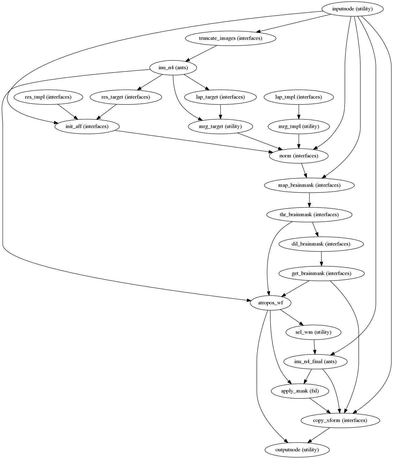
Next, the T1w reference is skull-stripped using a Nipype implementation of the antsBrainExtraction.sh tool (ANTs), which is an atlas-based brain extraction workflow:

(Source code, png, svg, pdf)

An example of brain extraction is shown below:

Brain extraction

Once the brain mask is computed, FSL fast is used for brain tissue segmentation.

Brain tissue segmentation

Finally, spatial normalization to standard spaces is performed using ANTs’ antsRegistration in a multiscale, mutual-information based, nonlinear registration scheme. See Standard and nonstandard spaces for more information on how standard and nonstandard spaces can be set to resample the preprocessed data onto the final output spaces.

Animation showing spatial normalization of T1w onto the MNI152NLin2009cAsym template.

ASL preprocessing

init_asl_preproc_wf()

(Source code)

Preprocessing of ASL files is split into multiple sub-workflows described below.

Processing GE data

ASLPrep can process data from any of the big three manufacturers (Siemens, Philips, GE), but GE ASL protocols are unique in that they typically only produce a single deltaM or CBF volume (optionally along with an M0 volume).

For these short sequences, ASLPrep performs many of the same steps as for a longer sequence, but certain steps are dropped, including motion correction and slice timing correction. Additionally, SCORE/SCRUB cannot be used with these short sequences, as the denoising method requires a long time series from which to identify outliers.

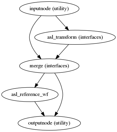
ASL reference image estimation

init_asl_reference_wf()

(Source code, png, svg, pdf)

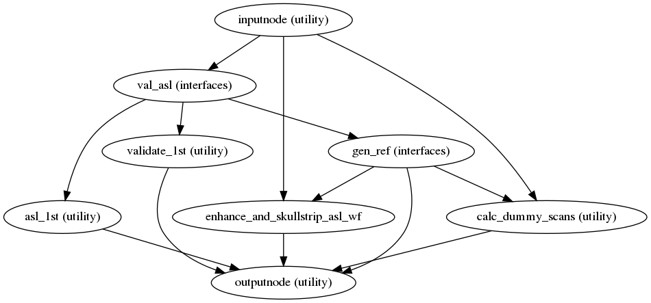
This workflow estimates a reference image for an ASL series. The reference image is then used to calculate a brain mask for the ASL signal using NiWorkflow’s init_enhance_and_skullstrip_asl_wf(). Subsequently, the reference image is fed to the head-motion estimation workflow and the registration workflow to map the ASL series onto the T1w image of the same subject.

Calculation of a brain mask from the ASL series.

Head-motion estimation

init_asl_hmc_wf()

(Source code, png, svg, pdf)

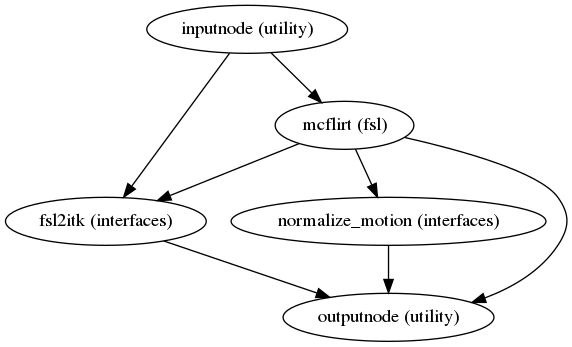
Using the previously estimated reference scan, FSL mcflirt or AFNI 3dvolreg is used to estimate head-motion. As a result, one rigid-body transform with respect to the reference image is written for each ASL time-step. Additionally, a list of 6-parameters (three rotations and three translations) per time-step is written and fed to the confounds workflow, for a more accurate estimation of head-motion.

Slice time correction

init_asl_stc_wf()

(Source code)

If the SliceTiming field is available within the input dataset metadata, this workflow performs slice time correction prior to other signal resampling processes. Slice time correction is performed using AFNI 3dTShift. All slices are realigned in time to the middle of each TR.

Slice time correction can be disabled with the --ignore slicetiming command line argument.

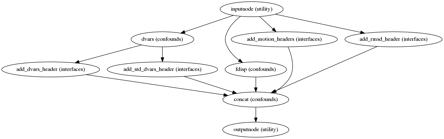
Confounds estimation

init_asl_confs_wf()

(Source code, png, svg, pdf)

Calculated confounds include framewise displacement, 6 motion parameters, and DVARS.

Susceptibility Distortion Correction (SDC)

One of the major problems that affects EPI data is the spatial distortion caused by the inhomogeneity of the field inside the scanner. Please refer to Susceptibility Distortion Correction (SDC) for details on the available workflows.

Applying susceptibility-derived distortion correction, based on fieldmap estimation

See also SDCFlows’ init_sdc_estimate_wf()

Preprocessed ASL in native space

init_asl_preproc_trans_wf()

(Source code, png, svg, pdf)

A new preproc ASL series is generated from either the slice-timing corrected data or the original data (if STC was not applied) in the original space. All volumes in the ASL series are resampled in their native space by concatenating the mappings found in previous correction workflows (HMC and SDC, if executed) for a one-shot interpolation process. Interpolation uses a Lanczos kernel.

The preprocessed ASL with label and control. The signal plots above the carpet plot are framewise diplacement (FD) and DVRAS.

CBF Computation in native space

init_cbf_compt_wf()

(Source code)

ASL data consist of multiple pairs of labeled and control images. ASLPrep first checks for proton density-weighted volume(s) (M0, sub-task_xxxx-acq-YYY_m0scan.nii.gz). In the absence of M0 images or an M0 estimate provided in the metadata, the average of control images is used as the reference image.

After preprocessing, the pairs of labeled and control images are subtracted:

\[ASL_{signal} = M_{C} - M_{L}\]

The CBF computation of either single or multiple PLD (post labelling delay) is done using a relatively simple model. For P/CASL (pseudo continuous ASL), CBF is calculated using a general kinetic model [3]:

\[CBF = \frac{ 6000 * \lambda * (M_{C} - M_{L})* e ^ \frac{ PLD }{ T1_{blood} } } {2 * \alpha * T1_{blood} * M_{0} * (1 - e^{\frac{ - \tau }{ T1_{blood} } }) }\]

Warning

As of 0.3.0, ASLPrep’s PASL support only extends to single-PLD data with either the QUIPSS or QUIPSSII BolusCutOffTechnique. We plan to support multi-PLD data, as well as Q2TIPS data, in the near future.

PASL (Pulsed ASL) is also computed by the QUIPSS model [4]:

\[CBF = \frac{ 6000 * \lambda * (M_{C} - M_{L})* e ^ \frac{ PLD }{ T1_{blood} } } {2 * \alpha * TI * M_{0}}\]

\(\tau\), \(\lambda\), and \(\alpha\) are label duration, brain-blood partition coefficient, and labeling efficiency, respectively. In the absence of any of these parameters, standard values are used based on the scan type and scanning parameters.

The computed CBF time series is shown in carpet plot below.

The carpet plot of computed CBF. The step plot above indicated the volume(s) marked by SCORE algorithm to be contaminated by noise.

Mean CBF is computed from the average of CBF timeseries.

Computed CBF maps

Warning

As of 0.3.0, ASLPrep has disabled multi-PLD support. We plan to properly support multi-PLD data in the near future.

For multi-PLD (Post Labeling Delay) ASL data, the CBF is first computed for each PLD and the weighted average CBF is computed over all PLDs at time = t [5].

\[CBF_{t} =\frac {\sum_{i}^{NPLDs} PLD_{i} * CBF_{i}} { \sum_{i}^{NPLDs} PLD_{i} }\]

Additional Denoising Options

ASLPrep includes the ability to denoise CBF with SCORE and SCRUB.

Structural Correlation based Outlier Rejection (SCORE) [6] detects and discards extreme outliers in the CBF volume(s) from the CBF time series. SCORE first discards CBF volumes whose CBF within grey matter (GM) means are 2.5 standard deviations away from the median of the CBF within GM. Next, it iteratively removes volumes that are most structurally correlated to the intermediate mean CBF map unless the variance within each tissue type starts increasing (which implies an effect of white noise removal as opposed to outlier rejection).

The mean CBF after denoising by SCORE is plotted below

Computed CBF maps denoised by SCORE

After discarding extreme outlier CBF volume(s) (if present) by SCORE, SCRUB (Structural Correlation with RobUst Bayesian) uses robust Bayesian estimation of CBF using iterative reweighted least square method [7] to denoise CBF. The SCRUB algorithm is described below:

\[ \begin{align}\begin{aligned}CBF_{SCRUB} = \arg\max_{\theta} \sum_{t=1}^N \rho(CBF_{t} -\theta) + \lambda(\theta -\mu)^2\\\mu =\sum_{i \in Tissue type} p *\mu_{i}\end{aligned}\end{align} \]

\(CBF_{t}\), \(\mu\), \(\theta\), and \(p\) equal CBF time series (after any extreme outliers are discarded by SCORE), mean CBF, ratio of temporal variance at each voxel to overall variance of all voxels, and probability tissue maps, respectively. Other variables include \(\lambda\) and \(\rho\) that represent the weighting parameter and Tukey’s bisquare function, respectively.

An example of CBF denoised by SCRUB is shown below.

Computed CBF maps denoised by SCRUB

ASLPrep also includes option of CBF computation by Bayesian Inference for Arterial Spin Labeling (BASIL). BASIL also implements a simple kinetic model as described above, but using Bayesian Inference principles [8]. BASIL is mostly suitable for multi-PLD. It includes bolus arrival time estimation with spatial regularization [9] and the correction of partial volume effects [10].

The sample of BASIL CBF with spatial regularization is shown below:

Computed CBF maps by BASIL

The CBF map shown below is the result of partial volume corrected CBF computed by BASIL.

Partial volume corrected CBF maps by BASIL

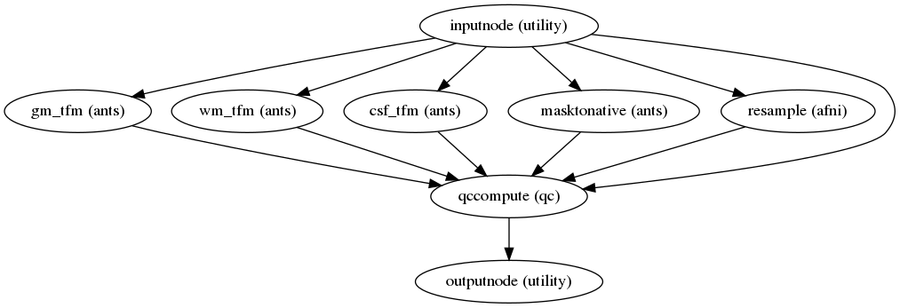
Quality control measures

init_compute_cbf_qc_wf()

(Source code, png, svg, pdf)

Quality control (QC) measures such as FD (framewise displacement), coregistration, normalization index, and quality evaluation index (QEI) are included for all CBF maps. The QEI [11] evaluates the quality of the computed CBF maps considering three factors: structural similarity, spatial variability, and percentage of voxels in GM with negative CBF.

ASL and CBF to T1w registration

init_asl_reg_wf()

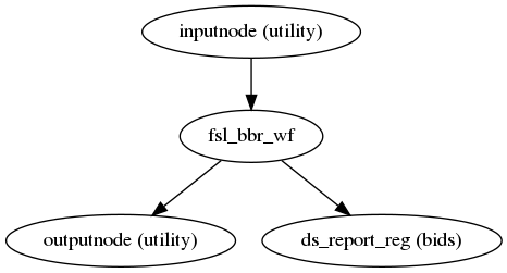
(Source code, png, svg, pdf)

ASLPrep uses the FSL BBR routine to calculate the alignment between each run’s ASL reference image and the reconstructed subject using the gray/white matter boundary.

Animation showing ASL to T1w registration.

FSL flirt is run with the BBR cost function, using the fast segmentation to establish the gray/white matter boundary. After BBR is run, the resulting affine transform will be compared to the initial transform found by flirt. Excessive deviation will result in rejection of the BBR refinement and acceptance of the original affine registration. The computed CBF is registered to T1w using the transformation from ASL-T1w registration.

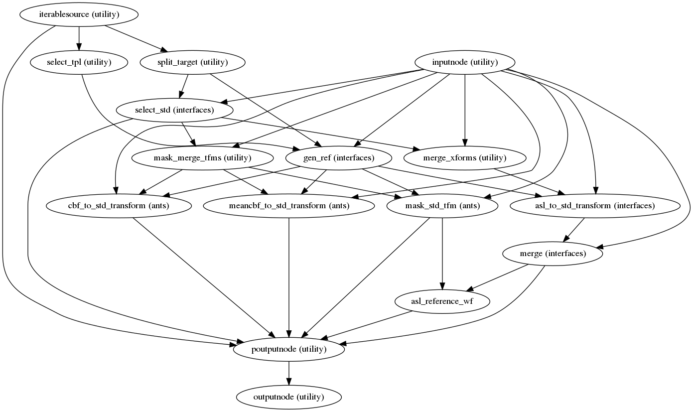
Resampling ASL and CBF runs onto standard spaces

init_asl_std_trans_wf()

(Source code, png, svg, pdf)

This sub-workflow concatenates the transforms calculated upstream (see Head-motion estimation, Susceptibility Distortion Correction (SDC)) if fieldmaps are available, and an anatomical-to-standard transform from Structural Preprocessing to map the ASL and CBF images to the standard spaces is given by the --output-spaces argument (see Standard and nonstandard spaces). It also maps the T1w-based mask to each of those standard spaces.

Transforms are concatenated and applied all at once, with one interpolation (Lanczos) step, so as little information is lost as possible.

References

[1]

Azeez Adebimpe, Maxwell Bertolero, Sudipto Dolui, Matthew Cieslak, Kristin Murtha, Erica B Baller, Bradley Boeve, Adam Boxer, Ellyn R Butler, Phil Cook, and others. Aslprep: a platform for processing of arterial spin labeled mri and quantification of regional brain perfusion. Nature methods, 19(6):683–686, 2022.

[2]

Azeez Adebimpe, Maxwell Bertolero, Kristin Murtha, Andrew Ross, Matt Flounders, Ellyn Butler, Matt Cieslak, Sydney Covitz, and Tinashe Michael Tapera. Aslprep <version>. Software, 2023. URL: https://doi.org/10.5281/zenodo.3759082, doi:10.5281/zenodo.3759082.

[3]

R. B. Buxton, L. R. Frank, E. C. Wong, B. Siewert, S. Warach, and R. R. Edelman. A general kinetic model for quantitative perfusion imaging with arterial spin labeling. Magn Reson Med., 40(3):383–396, September 1998. doi:10.1002/mrm.1910400308.

[4]

Eric C Wong, Richard B Buxton, and Lawrence R Frank. Quantitative imaging of perfusion using a single subtraction (quipss and quipss ii). Magnetic resonance in medicine, 39(5):702–708, 1998.

[5]

Weiying Dai, Philip M Robson, Ajit Shankaranarayanan, and David C Alsop. Reduced resolution transit delay prescan for quantitative continuous arterial spin labeling perfusion imaging. Magnetic resonance in medicine, 67(5):1252–1265, 2012.

[6]

Sudipto Dolui, Ze Wang, Russell T. Shinohara, David A. Wolk, John A. Detre, and for the Alzheimer’s Disease Neuroimaging Initiative. Structural Correlation-based Outlier Rejection (SCORE) algorithm for arterial spin labeling time series: SCORE: Denoising Algorithm for ASL. Journal of Magnetic Resonance Imaging, 45(6):1786–1797, June 2017. URL: http://doi.wiley.com/10.1002/jmri.25436 (visited on 2020-04-13), doi:10.1002/jmri.25436.

[7]

Sudipto Dolui, David A. Wolk, David A. Wolk, and John A. Detre. Scrub: a structural correlation and empirical robust bayesian method for asl data. International Society for Magnetic Resonance in Medicine, 2016. doi:http://archive.ismrm.org/2016/2880.html.

[8]

Michael A. Chappell, Adrian R. Groves, Brandon Whitcher, and Mark W. Woolrich. Variational bayesian inference for a nonlinear forward model. IEEE Transactions on Signal Processing, 2009. doi:10.1109/TSP.2008.2005752.

[9]

Adrian R Groves, Michael A Chappell, and Mark W Woolrich. Combined spatial and non-spatial prior for inference on mri time-series. Neuroimage, 45(3):795–809, 2009.

[10]

M. A. Chappell, A. R. Groves, B. J. MacIntosh, M. J. Donahue, P. Jezzard, and M. W. Woolrich. Partial volume correction of multiple inversion time arterial spin labeling MRI data. Magnetic Resonance in Medicine, 65(4):1173–1183, April 2011. doi:10.1002/mrm.22641.

[11]

Sudipto Dolui, Ronald Wolf, Seyed Ali Nabavizadeh, David A. Wolk, and John A. Detre. Automated quality evaluation index for 2d asl cbf maps. International Society for Magnetic Resonance in Medicine, 2016. doi:http://indexsmart.mirasmart.com/ISMRM2017/PDFfiles/0682.html.